So over the past couple of weeks I’ve been working on a little project called Demosaic. It’s a little online demo that interpolates image data from (simulated) raw sensor output, similar to what almost every digital camera used today has to do.
http://www.thedailynathan.com/demosaic/
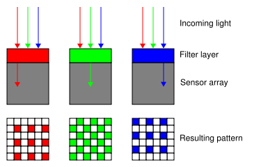
The core of the problem is that most digital cameras today make use of a color filter array, or CFA, in order to differentiate intensities based on wavelength, and thereby derive color. CFAs basically layer different color filters over each photodetector, only allowing that color light through and thereby isolating that intensity. By far the most common type of CFA used today is the Bayer filter, although many other variants exist.

Diagram of a Bayer pattern sensor
One of the downsides of using a CFA is that each photodetector, which normally corresponds to a pixel location in the final image, only detects light intensity for one wavelength range. So a blue-filtered detector will record exactly how much blue light was at the location, but has no idea how much red or green light there might be, for instance.
Digital cameras must therefore interpolate the missing data based on values recorded at nearby photodetectors, in a process known as “demosaicing”. Lots of different algorithms exist, with different tradeoffs in speed, quality, and suitability for different subject matter.
I developed the Demosaic demo as a sort of off-shoot of a broader research report I did on color detection for electronic image sensors for my Electrical Engineering 119 (EE119) optical engineering course at UC Berkeley. (That’ll get posted soon as well, probably in a few installments and after I get it reviewed and edited a few times.) Demosaic takes a test Bayer-pattern image (containing only the red, green, or blue values recorded at each location) and renders it into a final image using a variety of different algorithms.
As an example, here’s an original test image (images magnified 3x for clarity):

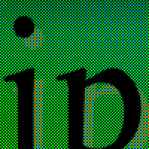
And here’s the raw Bayer data for the image. Every pixel is encoded with just a green, red, or blue value denoting the intensity of that color. To get a final image, we have to guess blue and red values at every green pixel, green and blue values at every red pixel, and so on.

One of the most basic ways to interpolate the information is to simply take an average (arithmetic mean) of the surrounding pixels. This is known as bilinear interpolatin, and produces a result like this:

Not terrible, especially as bilinear interpolation is just about the fastest algorithm out there (after nearest neighbor interpolation, which simply picks a single nearby pixel). The demosaicing artifacts are readily noticeable, however – color artifacting at white/black transitions, and “zipper” pattern artifacting along edges. Needless to say, this really isn’t all that acceptable for serious imaging applications.
Here’s another example with a more advanced algorithm known as Edge-sensing bilinear. This is an adaptive algorithm, which actually analyzes the image for local spatial features (in this case, harsh intensity transitions, or “edges”) and interpolates the data based on this context.

While not perfect, you can see this algorithm gets rid of many of the artifacts present in simple non-adaptive bilinear interpoltion. The zipper pattern artifacting has mostly disappeared, and the color artifacts at black/white transitions is also less apparent. As a tradeoff, however, this edge-sensing algorithm comes at a greater computational cost compared to simple bilinear interpolation.
To learn more about the different algorithms and run side-by-side comparisons, check out the Demosaic site. Also feel free to upload your own custom images to see how the algorithms perform on different types of image content.
Tags: Bayer, bayer filter, bayer pattern, color filter array, demosaic, demosaicing, interpolation, RGB


